Gallery II.

Single participant decision support

Academic design: the principle | parameters of target mixture

Comparative example: system | results of designs | dilemma of industrial design

Fig. 1 Academic design: Identified static mixture (left) is composed by three components. Minimizing its K-L divergence from the target mixture (middle) results in the advisory mixture (right).

Fig. 2 Academic design: Effect of changes of the target mean to the advisory mixture.

Fig. 3 Academic design: Effect of changes of the target variances to the advisory mixture.

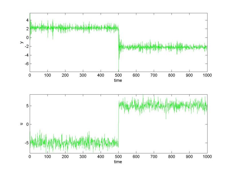
A simple comparative example

Let the system be defined by equations

Fig. 4 Time plots of the system output and input.

A dynamic mixture identified from data [y u] is composed by 8 components which attempt to model both modes of the system compromisingly. (There would be just 2 components for a deterministic system). The given target values for y* = 2.5 and u* = 0, represent the requirement to keep the output close to the mean of the 1^st mode with the minimal control effort. Variances for the target mixture are derived for each k from a component of the identified mixture which is the closest to actual data. Following figure compares results of academic, industrial and simultaneous designs.

Fig. 5 Comparison of three design methods on a simple example. Original data are plotted in green, result of the academic design in blue, industrial design in cyan and simultaneous in red. The target is drawn by a dotted black line.

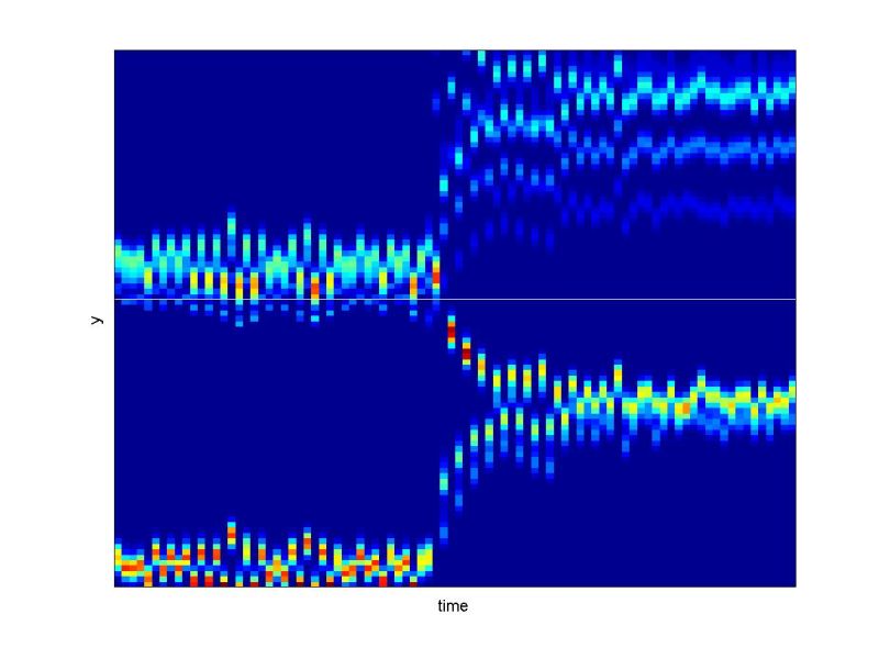
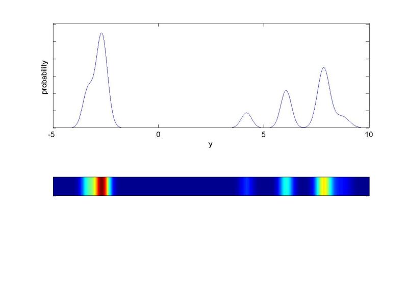
Academic design(blue) just changes components weights – value of u does not mean an ordinary control setpoint here but represents the weighted mean of used components. The result corresponds to the original data (green) for the 1^st mode while the expected output y is far from the target for the 2nd mode although closer than the original data.

Industrial design (cyan) meets the requirement for minimal values of control but expected output y for the 1^st mode is unsatisfactory. It is given by engaging all of the components with original weights. „Dilemma“ of the design is depicted on the following figure where probability distribution is mapped into colors for particular steps of k.

Fig. 6 „Dilemma" of the industrial design. The design uses original weights of all components implying considerable difference of expected output from the target (while line) for some or all modes. Distribution of the advisory mixture projected to the output for particular steps k is depicted by different colors according to the mapping shown on the following figure.

Simultaneous design (red) provides the best result for this case. Components with re-calculated weights are used for evaluation of recommendations of the control setpoints.

Fig. 7 Mapping of colors for depiction of the probability distribution.

It is appropriate to mention that the considered example just illustrates the approach the potential of which can be exploited for complex multidimensional and multimodal systems. For this system the target could be easily reached by the “normal” optimal control design.