Mixture identification - picture gallery

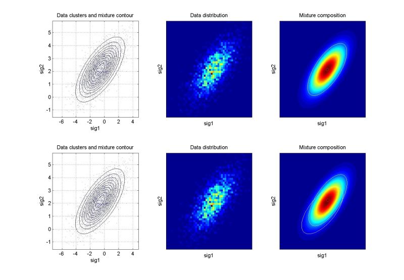
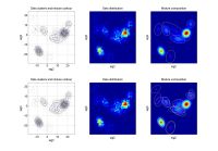
Plot rows in the following pictures correspond to the first or second identification runs respectively. Particular left plot shows data distribution and contour of the identified mixture. Middle plot depicts two-dimensional histogram of relative data frequency (empirical probability distribution) - the mixture should be similar to it. Right plot shows mixture composition. Two-dimensional projections are used for multidimensional cases.
Further criteria for evaluation of identification quality are based on comparison of calculated estimation likelihood and – for dynamic mixtures – on evaluation of prediction errors. Further information are or will be available on Links and articles page.

Meaning of identifiers in following tables: ndat - number of data samples, ndim – number of data channels (dimensions), ncom – number of components for simulating mixtures.
It is stated for multidimensional mixtures (ndim > 2) which dimensions are used for a 2-D projection.

Click on a plot to enlarge a picture.

Simulated data – static mixtures

Experiments with simulated data are advantageous for basic testing of algorithms as there is known “what should come out”.

Simulated data – static mixtures
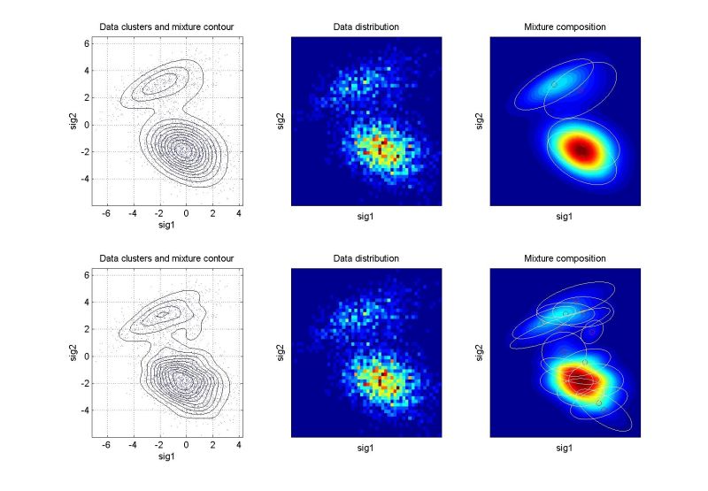
ndat=3000, ndim=2, ncom=1 The simplest case, the simulating mixture was composed by a single component. Identified well, the 2nd run does not bring anything new.	ndat=3000, ndim=2, ncom=2 The simulating mixture created by 2 adjacent components. The mixture from the 2nd run has too much components.
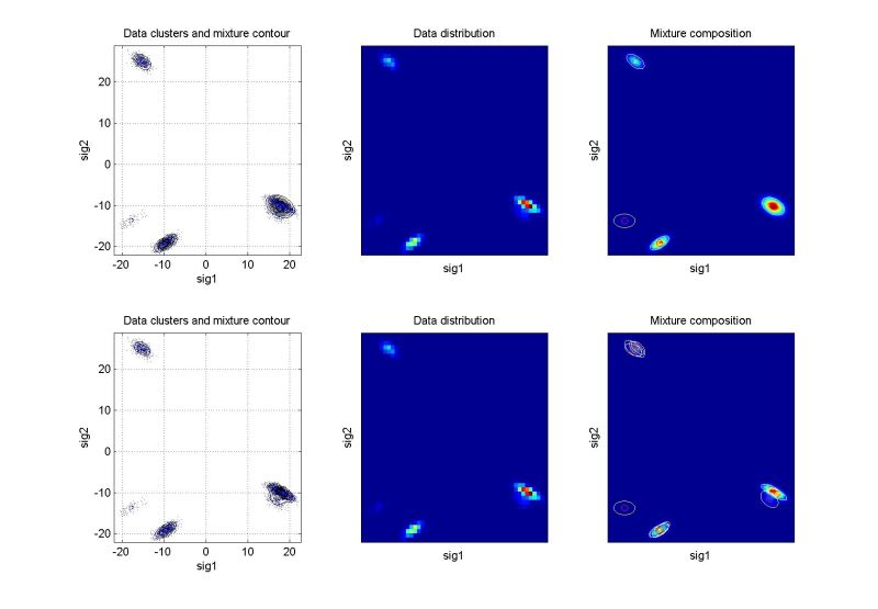
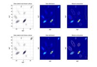
ndat=3000, ndim=2, ncom=5 The simulating mixture created by 5 isolated components. Good identification, 2nd run slightly better.	ndat=3000, ndim=2, ncom=5 The simulating mixture created by 5 adjacent components. The mixture from the 2nd run has too much components.
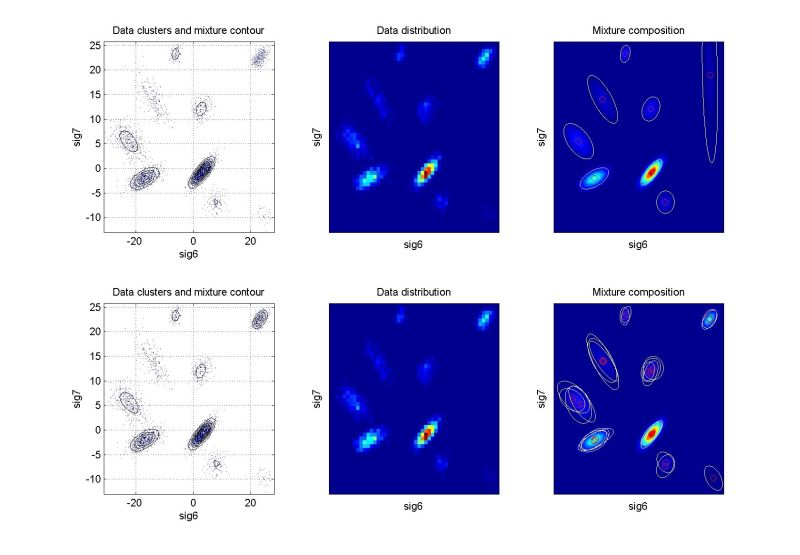
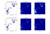
ndat=3000, ndim=9, ncom=9, projection 2-3 The simulating mixture created by 9 isolated components. Good identification, 2nd run slightly better. More components then necessary after the 2nd run.	ndat=3000, ndim=9, ncom=9, projection 6-7 Another projection of the foregoing mixture.

Simulated data – dynamic mixtures

Chronological succession of samples plays a key role for a dynamic mixture. Therefore the particular data sample must be given for the mixture projection. Dynamic mixtures are used for n-step ahead predictions.

Following picture shows an example of a dynamic mixture, which was identified from simulated data with the first order dynamics. Current data point moves around a circle for illustration.

Real data

Real data – static mixtures
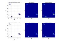
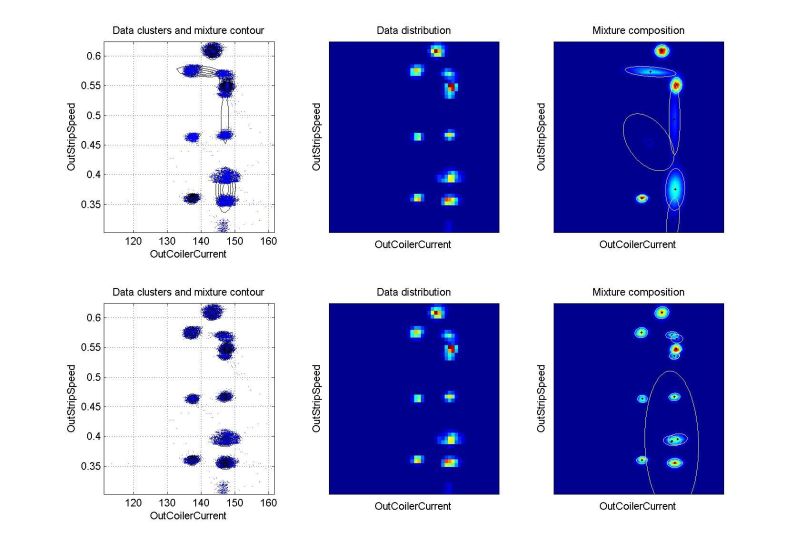
ndat=30000, ndim=2 Rolling mill data: values of electric currents for separated passes make isolated data clusters. 2nd run brings significant improvement.	ndat=30000, ndim=10 Rolling mill data: electric current of the output coiler drive against output strip speed. Vertical arrangement of data clusters made by simple distribution of the 1st signal channel. Good result.
ndat=30000, ndim=10 Rolling mill data: electric current of the main mill drive against output strip tension. Good result.

Real data – dynamic mixtures

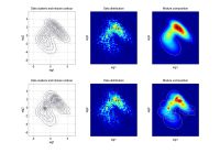
ndat=30000, ndim=10 Dynamic mixturesRolling mill data: projection of output strip tension against output strip thickness deviation. Empirical data distribution on the left plot followed by three projections for different values of time.